Lecture 1
- Image processing requires 3 main steps
- Capturing the image - Using Sensors
- Cameras use a sensor such as a CCD that image light falls onto using optics
- Low end cameras use a CFA that filters out light from a scene and each pixel is captured as either red, green or blue
- higher end camera use a dichroic filter (filters out two out of three colors) and have three chips. Three values captured at each pixel
- Digitization
- Images ae stored as a function of x and y along with a function of time if necessary. The intensity at each position is measured as an integer or a vector of 3 values depending on the type of imafe
- Storage
- Capturing the image - Using Sensors
- Video Sampling / Temporal Resolution (Framerate)
- Higher framerates at 50-60 fps produce smooth motion
- Progressive sampling samples each row, but interlaced sampling alternates the rows and columns to mimic smooth motion
- Spatial Resolution (no. of pixels)
- Perceived Resolution (Smallest details that can be resolved. Depends on the viewing distance and display)
Lecture 2
- Image Perception - The human eye perceives light by the product of the incident light and the reflectivity of the surface
- Photo receptors in the eye
- Cones (Photopic Vision)
- visual response to higher 5 to 6 orders of magnitude of illumination
- Rods (Scoptic Vision)
- Visual response of lower several orders of magnitude of illumination
- Cones (Photopic Vision)
- The luminance of an object is the product of it's light distribution
and a product of the relative luminous efficiency of the HVS - The luminance of an object is independent of the surrounding objects
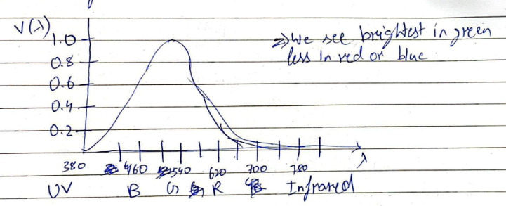
- The brightness/apparent brightness of an object is the perceived luminance* and depends on the luminance of the surroundings
- Contrast Sensitivity is when we can notice a brighter object from it's bright surroundings
where the is the just noticeable difference required from its surroundings L - Weber's Law -
and equal increments in the log of luminance should be perceived to be equally different 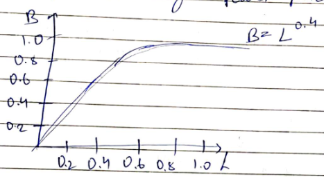
- Mach Bands are when in brightness according to our eyes the HVS overshoots around the boundaries of different intensity instead of following the actual change
- There is a drop before the change and an overshoot after
Lecture 3
- Definitions
- Visual Acuity - the ability to detect spatial details
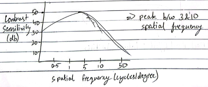
- Contrast Sensitivity - How visual acuity can change with spatial frequency (change in brightness)
- Modulation Transfer Function
- Mach Band Effect measures the response of the HVS in visual coordinates and the fourier transform of the impulse response gives the frequency response which can give the MTF
- This can also be directly measured by taking a sinusoidal grating of varying contrast ratio from maximum to minimum
- The shape is a band pass filter
- HVS is most sensitive to horizontal and vertical images
- Spatial Frequency refers to the number of oscillations in a grating. the eye can maximize edges and corners but it can detect only one or two intensity levels, so eye adapts to the average level of the image
- Image model means that the images are a function of the spatial coordinates that give the intensity of the image at that point
( ; , 0 is total absorption)
- Monochrome vision model (how our eyes perceive grayscale)
- Light comes in and passes through a low pass filter to become intensity. The intensity passes through the spectral response to become the luminance. The luminance reacts to the red/cone response to produce some contrast which through the process of lateral inhibition becomes brightness
-> ( , optics) -> -> Spectral Response ( )
->-> Red/Cone Response ( ) -> Contrast ( ) -> Lateral Inhibition ( ) ->
- Lateral inhibition is when the adjacent cells (cones/rods) limit the light energy coming into cell by subtraction
- Color Vision - Cones in the human retina contain three pigments
- S - Shortest for blue
- M - Middle for green
- R - longer for red
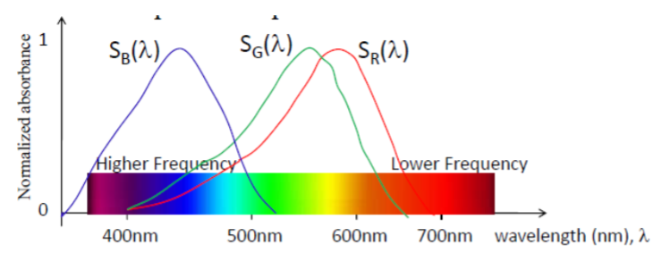
- Blue cones have higher color discrimination sensitivity
Lecture 4
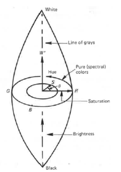
- Perceptual attributes of colour
- Brightness - Perceived Luminance
- Hue - redness, greenness
- Saturation - How much white light is added
- The spectral energy distribution of a "colored" light
will produce a color sensation that be described by "spectral responses" is the cone response and is the type of cone
- Color Matching function
- given a color we want to match it using a set of 3 primary light sources
- The proportion of mixing each color is
we want the new response to be perceived as color - We can define the i'th cone response by one unit of k'th primary as follows
- we combine and obtain
- Given an arbitrary color spectral distribution the primary sources and the sensitivity curves the quantities of each primary can be solved using
- where A is a matrix representing each spectral response to each primary and alpha is a vector of the spectral response to the given color
- given a color we want to match it using a set of 3 primary light sources
- Color calibration
- Typically the primary sources are matched to a known reference white light source
and defines the amount of k'th primary required to match it. - The tristimulus value of a color c is the relative amount of energy required to match a color
- Typically the primary sources are matched to a known reference white light source
- Chromaticity Diagram
- The chromaticity of a color is defined as
- only two chromaticity coordinates are required since
and these project the 3-d color space onto a 2-d plane - t1, and t2 represent the chrominance components of the color (hue and saturation)
- The entire space can be represented by coordinates t1, t2 and y which is a constant
- The chromaticity of a color is defined as
Lecture 5
- A signal is represented as
with and being the spatial coordinates and the height as - Special Impulses
which is 1 only when ( ) - Line impulses such as
- First quadrant step function
when and
- Basic 2-D operations
- Shifting a signal
(signal shifts up 1 and right 1)
- Flipping a signal
flip across x and y axis
- Flip and shift
shift every n steps to the right a flipped signal
- Shifting a signal
- Any general discrete 2-D signal can be written as a sum of shifted impulses
- A system is defined as a mathematical operator with an input and an output
- System properties
- Memoryless - If we call n1,n2 the present, then a system whose present output depends only on a present input
- Invertible - A system is invertible if for every output y there is only one unique input x
- Linear - If a system is based off of linearity (output doubles when input doubles)
- Shift Invariant - A system where any arbitrary shift in the input results in an identical shift in the output
- A stable system is one where every bounded input produces a bounded output
- In an LSI system the stability is equivalent to the impulse response being summable
- an impulse response is the output of an impulse passing through the system
Lecture 6
- Convolution
- If a discrete system is LSI then it's response to any arbitrary input can be computed using the convolution sum
- we multiple and add up the sums of the impulse response with the signal itself
- Properties
- Commutative
- Associative
- Distributive
- Convolution with a shifted impulse is the signal being shifted
- If a discrete system is LSI then it's response to any arbitrary input can be computed using the convolution sum
- DSFT
- The FT converts a signal from spatial domain to the frequency domain
- The 2D DSFT is periodic with
therefore we only need to calculate it for one period - The 2D DSFT can be written in terms of 1D DSFT by decomposing a set o f1-D DFT on all the column followed by another set of FTs on the rows (that are made from the prev. FT pass)
- The FT of the impulse response is the frequency response
- The inverse fourier transform of a frequency domain signal is
- Property
- A convolution in the space domain is a product in the frequency domain
- A shift in the original signal in the space domain equals a FT multiplied by the euler coeefecients
- The FT is separable into it's 1D parts
- The FT converts a signal from spatial domain to the frequency domain
Lecture 7
- Useful transform pairs
GPT help
Fourier Transform & Sampling Formula Sheet
1. Continuous Fourier Transform (CFT / CTFT)
1-D CFT
Inverse:
-
Continuous time
continuous frequency -
is continuous angular frequency in rad/s.
2-D CFT
Inverse:
2. Discrete-Time Fourier Transform (DTFT)
1-D DTFT
Inverse:
Periodicity
-
Discrete time
continuous, periodic frequency. -
Usually only need to consider
.
2-D DTFT
Inverse:
Periodicity:
3. Discrete Fourier Transform (DFT)
1-D
Inverse:
where:
DFT as Samples of the DTFT
2-D DFT
Inverse:
4. Important Fourier Transform Pairs
Constant
1-D
2-D
Constant signal
impulse at zero frequency (DC).
Impulse
1-D
Shifted:
2-D
Shifted:
Shifted impulse
complex exponential.
5. Complex Exponential
1-D
2-D
Complex exponential
one frequency impulse.
6. Cosine
Euler's identity:
1-D
2-D
Cosine
two impulses at .
7. Sine
Euler's identity:
1-D
Sine
two impulses with opposite signs/phases.
8. Gaussian
2-D:
Gaussian
Gaussian.
9. 45-Degree Impulse Line
Spatial line:
Frequency line:
10. Linearity
If:
then:
Transform each term separately and add the results.
11. Time/Spatial Shift
1-D
2-D
Shift in time/space
phase change in frequency.
12. Frequency Shift
1-D
2-D
Multiply by complex exponential
shift spectrum.
13. Convolution
For an LSI system:
Therefore:
and:
Convolution in time/space
multiplication in frequency.
14. Multiplication
1-D
2-D
Multiplication in time/space
convolution in frequency.
15. Complex Conjugation
For a real signal:
16. Sampling
Continuous
2-D:
Sampling Frequency
Angular Sampling Frequency
Continuous Frequency
2-D:
17. Nyquist / Aliasing
Nyquist criterion:
Angular frequency:
Since
2-D
If both conditions hold
no aliasing.
If spectral copies overlap
aliasing.
18. Sampling Creates Spectral Copies
For
General sampling period:
Spectral copies are separated by:
Sampling in time/space
periodic copies in frequency.
19. Reconstruction
Ideal sinc reconstruction:
where:
Important properties:
Therefore:
Perfect Reconstruction Condition
20. Unit Impulse
2-D:
Shifted:
21. Unit Step
Useful rectangular signal:
22. Delta Selection Property
2-D:
Delta "selects" the value at its location.
23. Important DFT Pairs
All Ones
Impulse
Shifted Impulse
Complex Exponential
24. Geometric Sum
Important DFT version:
25. Spatial Aliasing
Sampling an
For a
Sampling in frequency
periodic repetition/summing in space.
⭐ Highest Priority Formulas to Memorize
⭐ Fast Recognition Rules
-
Constant
impulse at DC. -
Impulse
constant spectrum. -
Shifted impulse
complex exponential. -
Complex exponential
one frequency impulse. -
Cosine
two frequency impulses. -
Gaussian
Gaussian. -
Spatial/time shift
phase in frequency. -
Multiplication by exponential
frequency shift. -
Convolution
multiplication. -
Sampling in time/space
repeated spectra. -
Sampling in frequency
repeated/summed spatial signal. -
Spectral overlap
aliasing. -
DTFT
continuous and -periodic in frequency. -
DFT
discrete frequency samples. -
Sinc interpolation
ideal reconstruction. -
Delta
set its argument equal to zero to find its location. -
Unit step
convert its argument into an inequality.